PTOPO - Topology of Parametric Curves

Elementary usage 

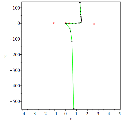
The easiest way to see the topology of a curve is to call the draw function with arguments the parametrization of the curve.

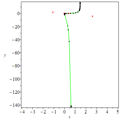
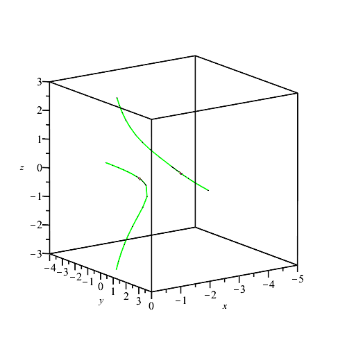
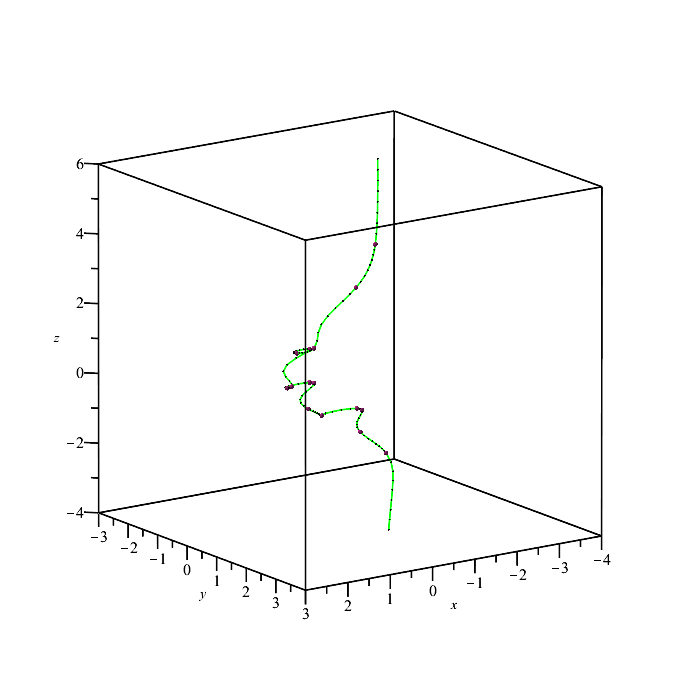
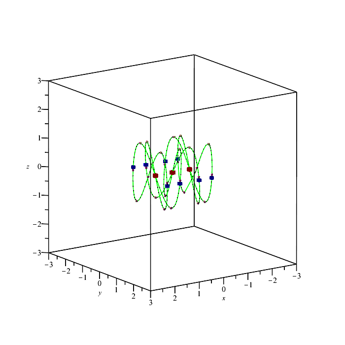
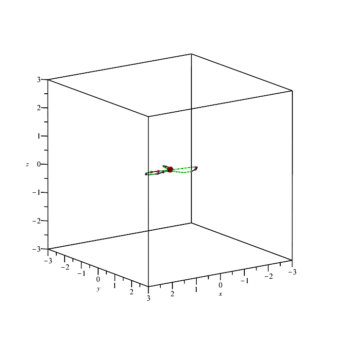
The output graph contains all the interesting points of the curve:
- in red box are the multiple points and cusps
- in red asterisk are the isolated points 

- in maroon circle are the extreme points with respect to the coordinate axis or planes
- in black circle are the points intersecting the bounding box and intermediate points sampled on the arcs

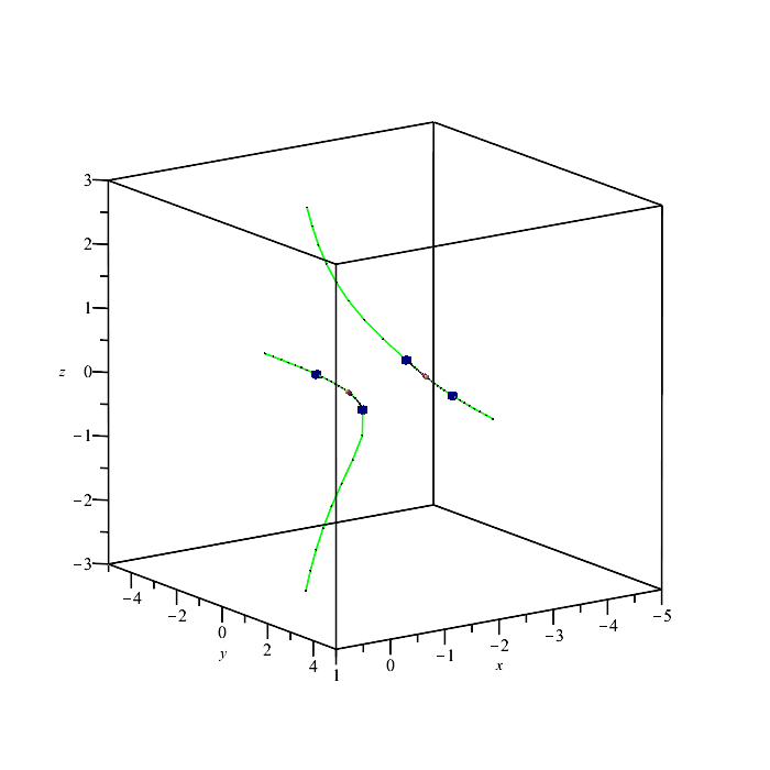
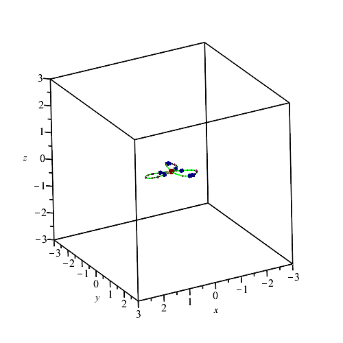
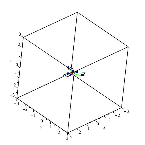
Additionally, for 3D curves, we perform a random projection of the curve to the plane. Then:
- in blue box are the apparent singularities (i.e., the sungularities of the projected curve)
- in khaki circle are the extreme points of the projected curve

Note that since the projection is random, the apparent singularities and the extreme points of the projected curve may differ among executions.  

>	p := [ (t^2 + 1)^2, 1]; q := [(t^4 + 1)^2, t^6]; PTOPO:-draw(p, q);

 

 

 

 

There is a point at infinity. We reparametrize.... ----****---- The parametrization is NOT proper  ----****----        The new parametrization is [1221025*(2*t+13)^2/(676*t^2+4368*t+14281)^2, -2197*(2*t+13)^3/(26*t-1)^3]  There is a point at infinity. We reparametrize.... ----****---- The parametrization is  proper  ----****---- * Compute topology... * Computing the poles...                           -- END * Computing point at infinity...                   -- END * Computing cusps and double points...             -- END * Computing extreme points...                      -- END * Computing the bounding box...                    -- END * Computing intersections with the bounding box... -- END * Topology computed -- END Computing points in branches Graph computed

 

>	phi := normal([ seq(p[i]/q[i], i=1..2)]); PTOPO:-draw(phi);

 

 

 

There is a point at infinity. We reparametrize.... ----****---- The parametrization is NOT proper  ----****----        The new parametrization is [197136*(t+3)^2/(288*t^2+840*t+1297)^2, -1728*(t+3)^3/(12*t-1)^3]  There is a point at infinity. We reparametrize.... ----****---- The parametrization is  proper  ----****---- * Compute topology... * Computing the poles...                           -- END * Computing point at infinity...                   -- END * Computing cusps and double points...             -- END * Computing extreme points...                      -- END * Computing the bounding box...                    -- END * Computing intersections with the bounding box... -- END * Topology computed -- END Computing points in branches Graph computed

 

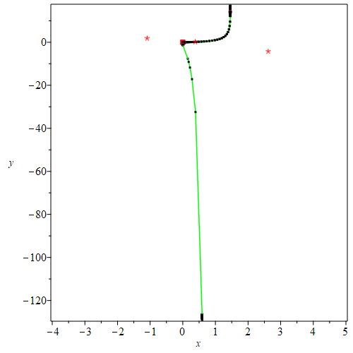
Additionally, we can provide the variable names and the number of points to be computed within the smooth arcs in the drawing. 

>	PTOPO:-draw(p, q,'t','s',5);

 

 

There is a point at infinity. We reparametrize.... ----****---- The parametrization is NOT proper  ----****----        The new parametrization is [30625*(2*t+7)^2/(196*t^2+672*t+1201)^2, -343*(2*t+7)^3/(14*t-1)^3]  There is a point at infinity. We reparametrize.... ----****---- The parametrization is  proper  ----****---- * Compute topology... * Computing the poles...                           -- END * Computing point at infinity...                   -- END * Computing cusps and double points...             -- END * Computing extreme points...                      -- END * Computing the bounding box...                    -- END * Computing intersections with the bounding box... -- END * Topology computed -- END Computing points in branches Graph computed

 

The function draw can be used in the same manner for the visualization of 3D parametric curves. 

>	p := [ -7*t^2-1, 1, t^3 ]; q := [ (t^2+1)^2, t^3, t^2+1 ]; PTOPO:-draw(p, q);

 

 

 

 

----****---- The parametrization is  proper  ----****---- * Compute topology... * Computing the poles...                           -- END * Computing point at infinity...                   -- END * Computing cusps and double points...             -- END * Computing extreme points...                      -- END * Computing the bounding box...                    -- END * Computing intersections with the bounding box... -- END * Topology computed -- END Computing points in branches Graph computed

 

>	phi := normal([seq(p[i]/q[i], i = 1 .. 3)]); PTOPO:-draw(phi);

 

 

 

----****---- The parametrization is  proper  ----****---- * Compute topology... * Computing the poles...                           -- END * Computing point at infinity...                   -- END * Computing cusps and double points...             -- END * Computing extreme points...                      -- END * Computing the bounding box...                    -- END * Computing intersections with the bounding box... -- END * Topology computed -- END Computing points in branches Graph computed

 

Similarly, we can provide the variable names and the number of points to be computed within the smooth arcs in the drawing. 

>	PTOPO:-draw(p,q,'t','s',5);

 

 

----****---- The parametrization is  proper  ----****---- * Compute topology... * Computing the poles...                           -- END * Computing point at infinity...                   -- END * Computing cusps and double points...             -- END * Computing extreme points...                      -- END * Computing the bounding box...                    -- END * Computing intersections with the bounding box... -- END * Topology computed -- END Computing points in branches Graph computed

 

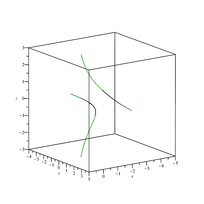A summary of the computed points is displayed by calling the point_summary function. 

>	PTOPO:-point_summary();

 

* Isolated points: * Poles:   :  t:  +0.000000   p * Extreme points: : [  -2.041667,  -1.656502,  -0.352148],   t:  -0.845154   e : [  -2.041667,  +1.656502,  +0.352148],   t:  +0.845154   e * Boundary points: : [  -0.552201,  -0.028364,  -3.000000],   t:  -3.279019   b : [  -1.936229,  -4.000000,  -0.178974],   t:  -0.629961   b : [  -1.936229,  +4.000000,  +0.178974],   t:  +0.629961   b : [  -0.552201,  +0.028364,  +3.000000],   t:  +3.279019   b * Cusps: * Multiple points: * Apparent singularities: * Extreme points of projected curve: : [  -1.784757,  -0.468961,  -0.802642],   t:  -1.287126   e(a) : [  -1.784757,  +0.468961,  +0.802642],   t:  +1.287126   e(a)

 

Initialize the parametrization 

The parametrization can be given as a pair of lists, the first containing the numerators and the second the denominators. 

>	p := [ t^2 + 1, 1]; q := [t^4 + 1, t^3];

 

 

	(2.1)

 

>	PTOPO:-parametrization(p, q);

 

There is a point at infinity. We reparametrize.... ----****---- The parametrization is  proper  ----****----

 

Alternatively, the parametrization can be given as a list containing the rational functions. 

>	phi := [(3*t^4+ 4*t^3 + 32*t^2 + 28*t + 99)/(t^2+t+7)*(t^2 + 1), ((t^2 + t + 7)^3)/((t+6)*(t^2 +1)^2)]; PTOPO:-parametrization(phi);

 

 

----****---- The parametrization is  proper  ----****----

 

We can see the current parametrization by calling the function without arguments. 

>	PTOPO:-parametrization();

 

 

	(2.2)

 

Both versions of the command accept  optional arguments for setting the variables. The defaults values are 't' and 's'. 

>	PTOPO:-parametrization(p, q, 't');

 

There is a point at infinity. We reparametrize.... ----****---- The parametrization is  proper  ----****----

 

>	PTOPO:-parametrization(p, q, 't', 's');

 

There is a point at infinity. We reparametrize.... ----****---- The parametrization is  proper  ----****----

 

Compute the topology 

To compute the topology of  the given parametric curve, we call  

>	PTOPO:-topology();

 

 

* Compute topology... * Computing the poles...                           -- END * Computing point at infinity...                   -- END * Computing cusps and double points...             -- END * Computing extreme points...                      -- END * Computing the bounding box...                    -- END * Computing intersections with the bounding box... -- END * Topology computed -- END
	(3.1)

 

Points of interest 

After the topology is computed we can see a summary of the points of interest: 

>	PTOPO:-point_summary();

 

* Isolated points: : [  -0.618034,  -0.485868]    i : [  -0.618034,  +0.485868]    i * Point at infinity: : [  +0.015865,  +0.001953] * Poles:   :  t:  -0.125000   p * Extreme points: : [  +1.207107,  +3.751141],   t:  -0.835837   e : [  +1.207107,  -3.751142],   t:  +0.479980   e * Boundary points: : [  +1.193395,  +5.999990],   t:  -0.725209   b : [  +1.193395,  -6.000000],   t:  +0.397946   b * Cusps: : [  +0.000000,  +0.000000],   t:  +8.000000   c * Multiple points:

 

The output contains the point in 2D (except for poles) and the correspodning parameter values (when applicable). The labels indicate:
- i for isolated points
- p for poles
- e for extreme points
- m for multiple points
- c for cusps
- b for boundary points 

We can get separately isolated points, point at infinity, poles, extreme points, multiple points and cusps. Moreover, we can see points intersecting the boundary of the box containing everything topologically interesting.  

>	PTOPO:-isolated_points();

 

* Isolated points: : [  -0.618034,  -0.485868]    i : [  -0.618034,  +0.485868]    i

 

>	PTOPO:-point_at_infinity();

 

* Point at infinity: : [  +0.015865,  +0.001953]

 

>	PTOPO:-poles();

 

* Poles:   :  t:  -0.125000   p

 

>	PTOPO:-extreme_points();

 

* Extreme points: : [  +1.207107,  +3.751141],   t:  -0.835837   e : [  +1.207107,  -3.751142],   t:  +0.479980   e

 

>	PTOPO:-multiple_points();

 

* Multiple points:

 

>	PTOPO:-cusps();

 

* Cusps: : [  +0.000000,  +0.000000],   t:  +8.000000   c

 

>	PTOPO:-boundary_points();

 

* Boundary points: : [  +1.193395,  +5.999990],   t:  -0.725209   b : [  +1.193395,  -6.000000],   t:  +0.397946   b

 

Similarly, for a 3D curve, we use the same command to get a summary of the points of interest: 

>	PTOPO:-parametrization([-3*t^2 + 1,(-3*t^2 + 1)*t,(-3*t^2 + 1)*t^3], [(t^2 + 1)^2,(t^2 + 1)^2,(t^2 + 1)^4]); PTOPO:-topology(): PTOPO:-point_summary();

 

There is a point at infinity. We reparametrize.... ----****---- The parametrization is  proper  ----****---- * Compute topology... * Computing the poles...                           -- END * Computing point at infinity...                   -- END * Computing cusps and double points...             -- END * Computing extreme points...                      -- END * Computing the bounding box...                    -- END * Computing intersections with the bounding box... -- END * Topology computed -- END * Isolated points: * Point at infinity: : [  -0.013196,  -0.197940,  -0.000872] * Poles:   * Extreme points: : [  -0.444803,  -0.880086,  -0.142633],   t:  -2.356043   e : [  -0.553188,  -0.794059,  -0.174681],   t:  -1.661045   e : [  -0.562500,  -0.726184,  -0.170199],   t:  -1.485514   e : [  +0.381313,  +0.153370,  +0.018383],   t:  -0.481801   e : [  +0.632303,  +0.184504,  +0.013341],   t:  -0.365576   e : [  +1.000000,  +0.000000,  +0.000000],   t:  -0.066667   e : [  +0.632303,  -0.184504,  -0.013341],   t:  +0.220835   e : [  +0.381313,  -0.153370,  -0.018383],   t:  +0.326786   e : [  -0.562500,  +0.726184,  +0.170199],   t:  +1.127305   e : [  -0.553188,  +0.794059,  +0.174681],   t:  +1.249215   e : [  -0.444803,  +0.880086,  +0.142633],   t:  +1.689126   e * Boundary points: * Cusps: * Multiple points: : [  +0.000000,  +0.000000,  +0.000000],   t:  -0.669797   m : [  +0.000000,  +0.000000,  +0.000000],   t: +15.000000   m : [  +0.000000,  -0.000000,  -0.000000],   t:  +0.491756   m * Apparent singularities: : [  -0.280212,  -0.799723,  -0.077885],   t:  -3.606940   a : [  -0.353553,  -0.853553,  -0.106694],   t:  -2.956764   a : [  -0.280212,  -0.209861,  -0.048313],   t:  -0.858465   a : [  +0.353553,  +0.146447,  +0.018306],   t:  -0.494536   a : [  +0.353553,  -0.146447,  -0.018306],   t:  +0.338208   a : [  -0.280212,  +0.209861,  +0.048313],   t:  +0.649824   a : [  -0.353553,  +0.853553,  +0.106694],   t:  +2.022096   a : [  -0.280212,  +0.799723,  +0.077885],   t:  +2.341768   a * Extreme points of projected curve: : [  -0.113251,  -0.555757,  -0.021274],   t:  -7.392439   e(a) : [  -0.562425,  -0.719427,  -0.169381],   t:  -1.471284   e(a) : [  +0.164384,  +0.081861,  +0.013034],   t:  -0.584044   e(a) : [  +0.839417,  +0.155036,  +0.004945],   t:  -0.254495   e(a) : [  +0.839417,  -0.155036,  -0.004945],   t:  +0.116593   e(a) : [  +0.164384,  -0.081861,  -0.013034],   t:  +0.417462   e(a) : [  -0.562425,  +0.719427,  +0.169381],   t:  +1.117212   e(a) : [  -0.113251,  +0.555757,  +0.021274],   t:  +3.647385   e(a)

 

In the point summary above, apparent singularities are labeled with "a", and extreme points of the projected curve with "e(a)".
We can get separately all the points of the interest with the following commands: 

>	PTOPO:-poles();

 

* Poles:

 

>	PTOPO:-point_at_infinity();

 

* Point at infinity: : [  -0.013196,  -0.197940,  -0.000872]

 

>	PTOPO:-extreme_points();

 

* Extreme points: : [  -0.444803,  -0.880086,  -0.142633],   t:  -2.356043   e : [  -0.553188,  -0.794059,  -0.174681],   t:  -1.661045   e : [  -0.562500,  -0.726184,  -0.170199],   t:  -1.485514   e : [  +0.381313,  +0.153370,  +0.018383],   t:  -0.481801   e : [  +0.632303,  +0.184504,  +0.013341],   t:  -0.365576   e : [  +1.000000,  +0.000000,  +0.000000],   t:  -0.066667   e : [  +0.632303,  -0.184504,  -0.013341],   t:  +0.220835   e : [  +0.381313,  -0.153370,  -0.018383],   t:  +0.326786   e : [  -0.562500,  +0.726184,  +0.170199],   t:  +1.127305   e : [  -0.553188,  +0.794059,  +0.174681],   t:  +1.249215   e : [  -0.444803,  +0.880086,  +0.142633],   t:  +1.689126   e

 

>	PTOPO:-multiple_points();

 

* Multiple points: : [  +0.000000,  +0.000000,  +0.000000],   t:  -0.669797   m : [  +0.000000,  +0.000000,  +0.000000],   t: +15.000000   m : [  +0.000000,  -0.000000,  -0.000000],   t:  +0.491756   m

 

>	PTOPO:-cusps();

 

* Cusps:

 

>	PTOPO:-apparent_singularities();

 

* Apparent singularities: : [  -0.280212,  -0.799723,  -0.077885],   t:  -3.606940   a : [  -0.353553,  -0.853553,  -0.106694],   t:  -2.956764   a : [  -0.280212,  -0.209861,  -0.048313],   t:  -0.858465   a : [  +0.353553,  +0.146447,  +0.018306],   t:  -0.494536   a : [  +0.353553,  -0.146447,  -0.018306],   t:  +0.338208   a : [  -0.280212,  +0.209861,  +0.048313],   t:  +0.649824   a : [  -0.353553,  +0.853553,  +0.106694],   t:  +2.022096   a : [  -0.280212,  +0.799723,  +0.077885],   t:  +2.341768   a

 

>	PTOPO:-extreme_points_2();

 

* Extreme points of projected curve: : [  -0.113251,  -0.555757,  -0.021274],   t:  -7.392439   e(a) : [  -0.562425,  -0.719427,  -0.169381],   t:  -1.471284   e(a) : [  +0.164384,  +0.081861,  +0.013034],   t:  -0.584044   e(a) : [  +0.839417,  +0.155036,  +0.004945],   t:  -0.254495   e(a) : [  +0.839417,  -0.155036,  -0.004945],   t:  +0.116593   e(a) : [  +0.164384,  -0.081861,  -0.013034],   t:  +0.417462   e(a) : [  -0.562425,  +0.719427,  +0.169381],   t:  +1.117212   e(a) : [  -0.113251,  +0.555757,  +0.021274],   t:  +3.647385   e(a)

 

Draw 

Finally, we can draw the topology of the curve.  

>	PTOPO:-draw();

 

 

Computing points in branches Graph computed

 

The draw command accepts one optional argument controling how many points should be computed in every arc. Increasing the number increases the computational cost but improves the drawing. Note that it does not affect the topological correctness of the drawing. 

>	PTOPO:-draw(4);

 

 

Computing points in branches Graph computed

 

Examples 

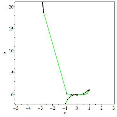
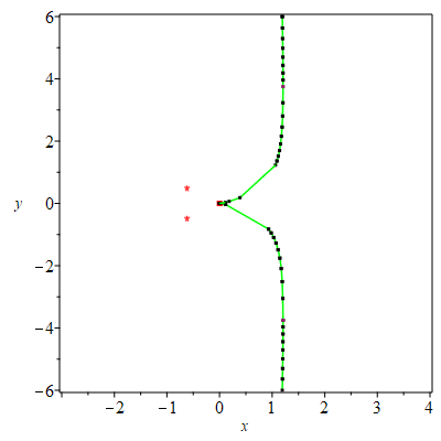
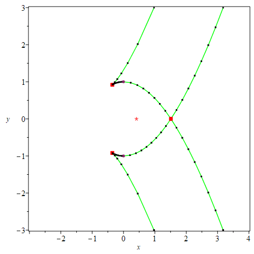
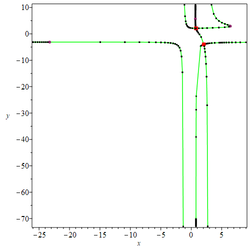
PTOPO comes with some examples ready to use. Some of the examples come from Alc�zar and D�az-Toca [CAGD'10]. 

>	PTOPO:-example_2d(1);

 

(6.1)

 

>	PTOPO:-draw(PTOPO:-example_2d(1));

 

 

There is a point at infinity. We reparametrize.... ----****---- The parametrization is  proper  ----****---- * Compute topology... * Computing the poles...                           -- END * Computing point at infinity...                   -- END * Computing cusps and double points...             -- END * Computing extreme points...                      -- END * Computing the bounding box...                    -- END * Computing intersections with the bounding box... -- END * Topology computed -- END Computing points in branches Graph computed

 

>	PTOPO:-draw(PTOPO:-example_2d(2));

 

 

There is a point at infinity. We reparametrize.... ----****---- The parametrization is  proper  ----****---- * Compute topology... * Computing the poles...                           -- END * Computing point at infinity...                   -- END * Computing cusps and double points...             -- END * Computing extreme points...                      -- END * Computing the bounding box...                    -- END * Computing intersections with the bounding box... -- END * Topology computed -- END Computing points in branches Graph computed

 

>	PTOPO:-draw(PTOPO:-example_2d(3));

 

 

----****---- The parametrization is  proper  ----****---- * Compute topology... * Computing the poles...                           -- END * Computing point at infinity...                   -- END * Computing cusps and double points...             -- END * Computing extreme points...                      -- END * Computing the bounding box...                    -- END * Computing intersections with the bounding box... -- END * Topology computed -- END Computing points in branches Graph computed

 

>	PTOPO:-draw(PTOPO:-example_2d(4));

 

 

There is a point at infinity. We reparametrize.... ----****---- The parametrization is  proper  ----****---- * Compute topology... * Computing the poles...                           -- END * Computing point at infinity...                   -- END * Computing cusps and double points...             -- END * Computing extreme points...                      -- END * Computing the bounding box...                    -- END * Computing intersections with the bounding box... -- END * Topology computed -- END Computing points in branches Graph computed

 

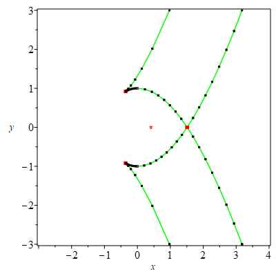
>	PTOPO:-draw(PTOPO:-example_2d(5));

 

 

----****---- The parametrization is  proper  ----****---- * Compute topology... * Computing the poles...                           -- END * Computing point at infinity...                   -- END * Computing cusps and double points...             -- END * Computing extreme points...                      -- END * Computing the bounding box...                    -- END * Computing intersections with the bounding box... -- END * Topology computed -- END Computing points in branches Graph computed

 

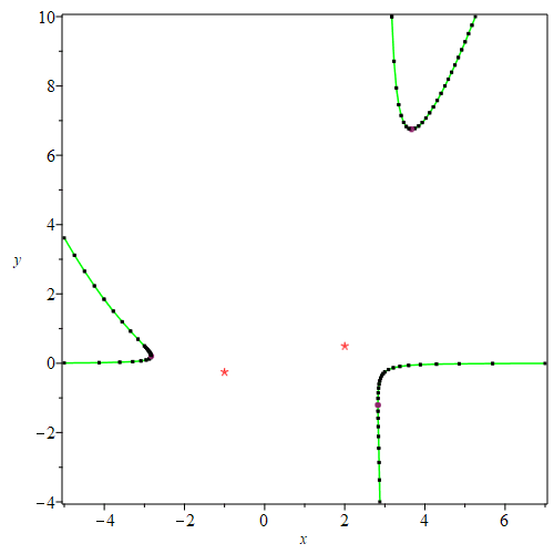
>	PTOPO:-draw(PTOPO:-example_2d(6));

 

 

----****---- The parametrization is NOT proper  ----****----        The new parametrization is [(-2*t^2+28*t-99)/(t-7), 1/(t-6)*(t-7)^3] ----****---- The parametrization is  proper  ----****---- * Compute topology... * Computing the poles...                           -- END * Computing point at infinity...                   -- END * Computing cusps and double points...             -- END * Computing extreme points...                      -- END * Computing the bounding box...                    -- END * Computing intersections with the bounding box... -- END * Topology computed -- END Computing points in branches Graph computed

 

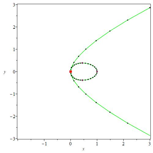
>	PTOPO:-draw(PTOPO:-example_2d(7)); PTOPO:-point_summary();

 

 

 

----****---- The parametrization is  proper  ----****---- * Compute topology... * Computing the poles...                           -- END * Computing point at infinity...                   -- END * Computing cusps and double points...             -- END * Computing extreme points...                      -- END * Computing the bounding box...                    -- END * Computing intersections with the bounding box... -- END * Topology computed -- END Computing points in branches Graph computed
* Isolated points: * Poles:   * Extreme points: : [  +0.444438,  +0.384900],   t:  -0.577354   e : [  +1.000000,  +0.000000],   t:  +0.000000   e : [  +0.444445,  -0.384900],   t:  +0.577350   e * Boundary points: : [  +3.002114,  -2.864220],   t:  -1.653076   b : [  +2.999841,  +2.862793],   t:  +1.652878   b * Cusps: * Multiple points: : [  +0.000000,  +0.000000],   t:  -1.000000   m : [  +0.000000,  +0.000000],   t:  +1.000000   m

 

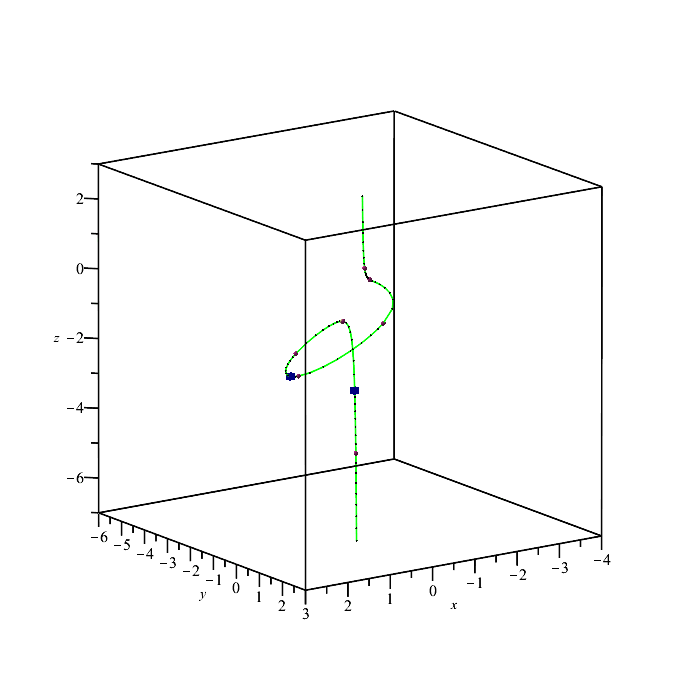
>	PTOPO:-draw(PTOPO:-example_3d(1));

 

 

----****---- The parametrization is  proper  ----****---- * Compute topology... * Computing the poles...                           -- END * Computing point at infinity...                   -- END * Computing cusps and double points...             -- END * Computing extreme points...                      -- END * Computing the bounding box...                    -- END * Computing intersections with the bounding box... -- END * Topology computed -- END Computing points in branches Graph computed

 

>	PTOPO:-draw(PTOPO:-example_3d(2));

 

 

----****---- The parametrization is  proper  ----****---- * Compute topology... * Computing the poles...                           -- END * Computing point at infinity...                   -- END * Computing cusps and double points...             -- END * Computing extreme points...                      -- END * Computing the bounding box...                    -- END * Computing intersections with the bounding box... -- END * Topology computed -- END Computing points in branches Graph computed

 

>	PTOPO:-draw(PTOPO:-example_3d(3));

 

 

There is a point at infinity. We reparametrize.... ----****---- The parametrization is  proper  ----****---- * Compute topology... * Computing the poles...                           -- END * Computing point at infinity...                   -- END * Computing cusps and double points...             -- END * Computing extreme points...                      -- END * Computing the bounding box...                    -- END * Computing intersections with the bounding box... -- END * Topology computed -- END Computing points in branches Graph computed

 

>	PTOPO:-draw(PTOPO:-example_3d(4));

 

 

There is a point at infinity. We reparametrize.... ----****---- The parametrization is  proper  ----****---- * Compute topology... * Computing the poles...                           -- END * Computing point at infinity...                   -- END * Computing cusps and double points...             -- END * Computing extreme points...                      -- END * Computing the bounding box...                    -- END * Computing intersections with the bounding box... -- END * Topology computed -- END Computing points in branches Graph computed

 

>